How Does Radar Work?

Fundamentally, millimeter wave (mmWave) radar devices transmit pulses of electromagnetic waves (called chirps) which reflect off of a target. These reflected signals are then captured and processed by the radar to determine the target’s range, velocity, and direction. Radar is a good fit for applications that require precise position and velocity measurements. Radar devices are capable of penetrating many materials at very low power consumption.

TI’s mmWave radar sensors implement frequency modulated continuous wave (FMCW) technology. A complete FMCW radar system includes:

Transmit (TX) and receive (RX) radio frequency (RF) components
Analog components such as clocking and filtering
Digital components such as analog-to-digital converters (ADCs), microcontrollers (MCUs) and digital signal processors (DSPs) Traditionally, these systems were implemented with discrete components, which increased power consumption and overall system cost. Due to the complexity of high frequency layout, system design was very difficult.

Texas Instruments (TI) has solved these challenges and designed complementary metal-oxide semiconductor (CMOS)-based mmWave radar devices that integrate TX-RF and RX-RF analog components such as clocking, and digital components such as the ADC, MCU and hardware accelerator onto the same package. Some families in TI’s mmWave sensor portfolio integrate a DSP for additional signal-processing capabilities.

Chirps

The signal transmitted by a FMCW radar is called a chirp. Figure 1 shows the lifecycle of a chirp from transmission to radar output.

Block diagram of an example radar's frontend processing chain — **Figure 1.** *Block diagram showing an example radar’s processing chain hardware.*

The chirp is generated by a synth and transmitted through the TX antenna.
The chirp bounces off of the target and is captured by the RX antenna.
The TX chirp and RX chirp are combined by a signal mixer to create an Intermediate Frequency signal
This Intermediate Frequency signal is processed by analog filters and converted to a digital signal
The Raw ADC data is either transferred off-chip or digitally processed on-chip to produce radar heatmap data, point-cloud data, or tracker/classifier output. (For more info on the different forms of radar data, visit the What Does Radar Data Look Like Module.)

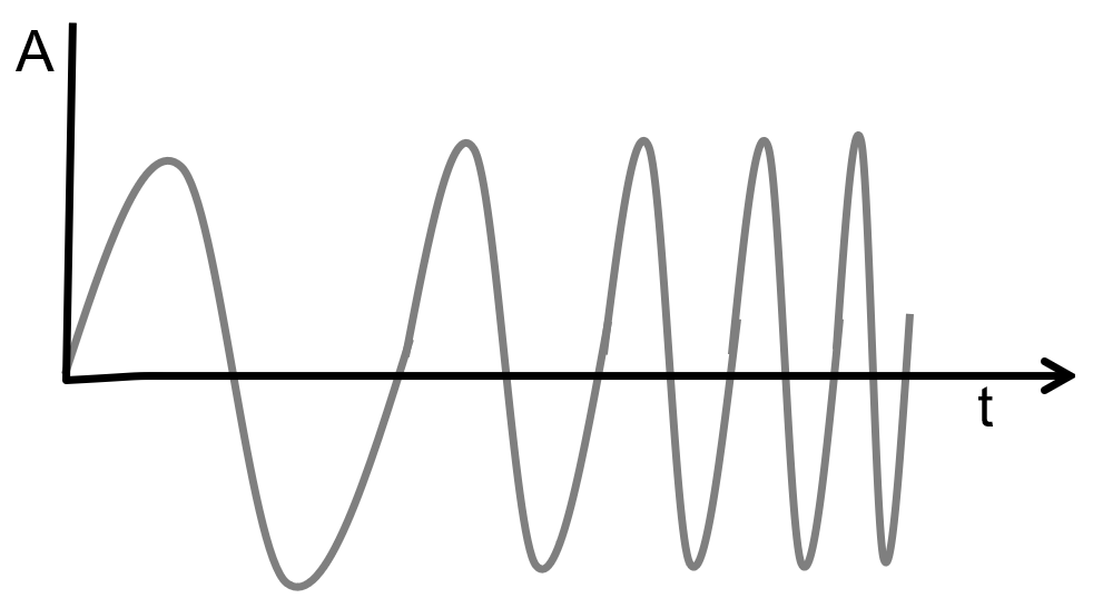
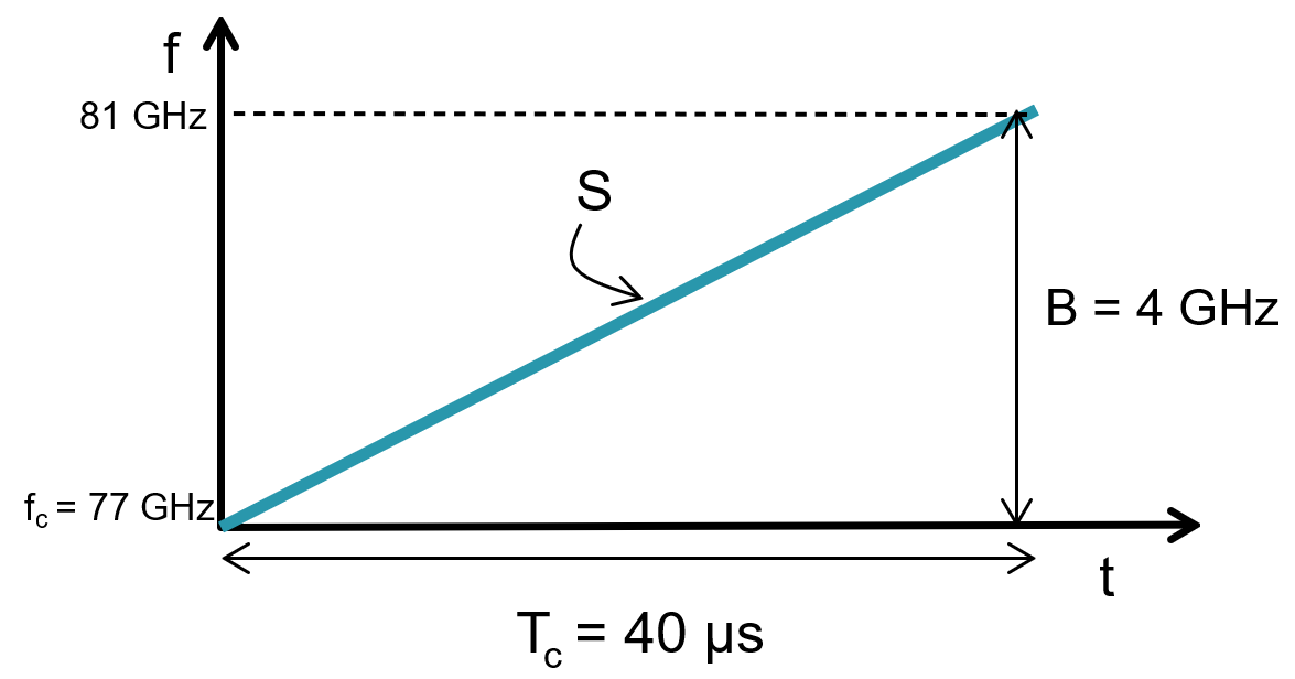
Figure 2 shows an FMCW chirp, which when plotted over time are a sine wave that increases in frequency. Figure 3 shows the same chirp signal, but with frequency plotted as a function of time. The chirp is characterized by a start frequency (f_c), frequency bandwidth (B), and chirp duration (T_c). The slope of the chirp (S) is just the rate of frequency change over time. As an example, Figure 3 has f_c = 77 GHz, B = 4 GHz, T_c = 40 μs and S = 100 MHz/μs.

**Figure 2.** *Example chirp plotted on amplitude vs. time axis.*

**Figure 3.** *Example chirp plotted on chirp frequency vs. time axis.*

Range Estimation

Once the chirp is generated, it must then be transmitted through one or more TX antennas. While the chirp is being transmitted, the RX antennas will be absorbing any signals that are reflected by objects in the area. Depending on the detected object’s movement or position, the reflected signal may have a different frequency or phase than the initial transmitted signal. Once the reflected signal is received by the RX antennas, processing can begin.

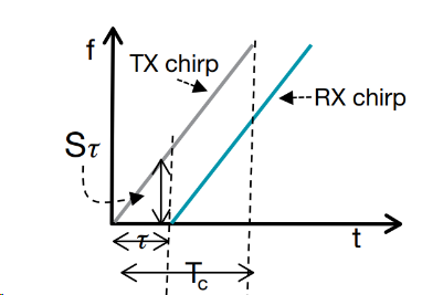
Figure 4 shows the transmitted TX signal and the received RX signal plotted on the same frequency vs time graph. The time difference T between the TX chirp and RX chirp corresponds to a frequency difference of S⋅t Hz between the TX chirp and RX chirp.

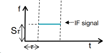
**Figure 4.** *Transmitted and received chirp plotted on the same frequency vs. time axis.*

This correlation is then visualizer in Figure 5, where the frequency of the RX signal is subtracted from the TX signal. This creates a new signal with a constant frequency that directly correlates to the distance between the radar and the detected object. The frequency that results from this subtraction is called the intermediate frequency, or IF signal. This subtraction of the TX chirp from the RX (mentioned in Figure 1)

**Figure 5.** *Intermediate frequency resulting from subtraction of RX chirp from TX chirp.*

To calculate range from the intermediate frequency, keep in mind that radar is a form of electromagnetic wave and therefore travels at the speed of light. The time delay from TX to RX can then be calculated by t=frac2⋅dc where d is distance traveled (multiplied by 2, since the signal travels to the object and back) and c is the speed of light. Since time delay is related to the chirp slope (S) and intermediate frequency (IF) by t=IF⋅S, distance can be determined by solving these two equations.

This process of creating an intermediate frequency is at the core of FMCW radar processing.

Velocity Estimation

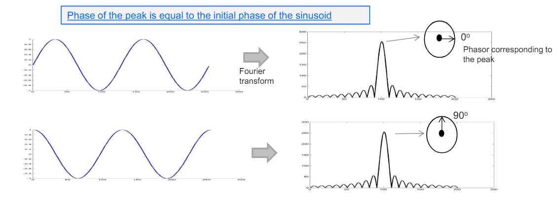
Radar can also be used to detect an object’s instantaneous velocity with a high degree of accuracy using the phase of the IF signal. Finding the phase of the IF signal is made possible through Fourier transforms. Fourier transforms are used to convert sinusoidal signals in the time domain into peaks in the frequency domain. Figure 6 shows the IF sinusoid being transformed into a frequency domain signal, which allows its frequency and its phase to be determined.

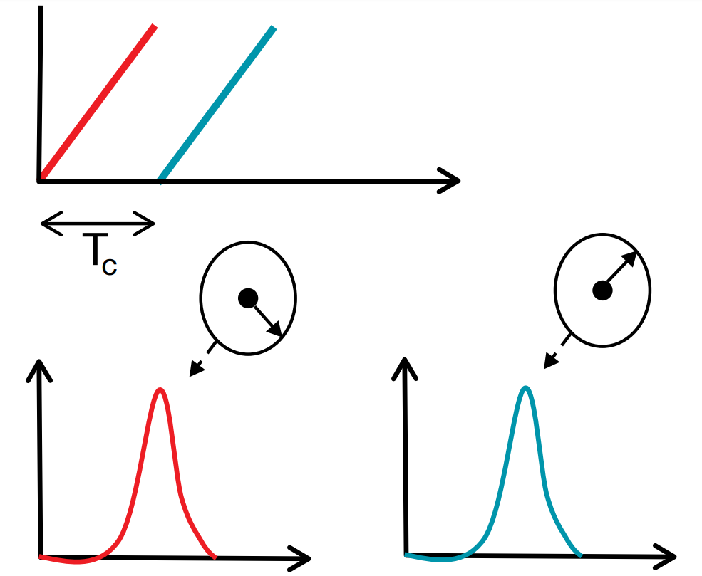
Fourier Transforming IF signal to determine frequency and phase. — **Figure 6.** *Fourier Transforming an IF signal to determine frequency and phase.*

While a single phase measurement is not sufficient to obtain meaningful data, the phase measurements from multiple chirps can be compared to measure small motions. Figure 7 shows an example of two chirps that are separated by T_c seconds to get two phase measurements.

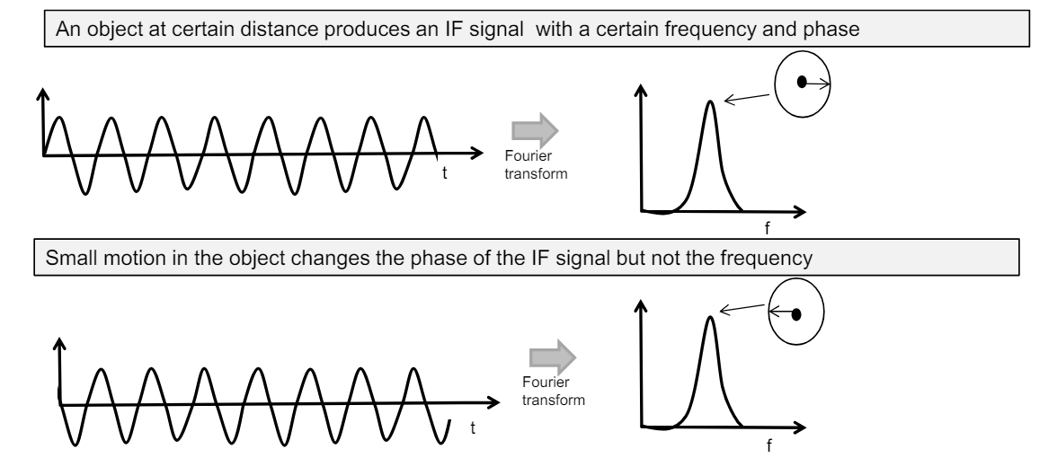
**Figure 7.** *Phase difference between the IF signals of two chirps.*

If the detected object is moving, the distance calculated from the second chirp will be different than the distance calculated from the first. This distance difference corresponds to a phase difference between the IF signals of the first and second chirp. Therefore, chirping at moving objects produces a measurable phase difference across multiple chirps.

**Figure 8.** *Phase difference between two chirps caused by velocity of detected object.*

Detecting an object’s position

While all measurements discussed so far (velocity, distance) have been one-dimensional, these same principles can be applied and built upon to determine the location of an object in 2D or 3D space.

The ability for a radar sensor to localize an object in 2D or 3D space is dependent on its number of antennas and their layout. Consider the system shown in Figure 9, which has one TX antenna but two RX antennas.

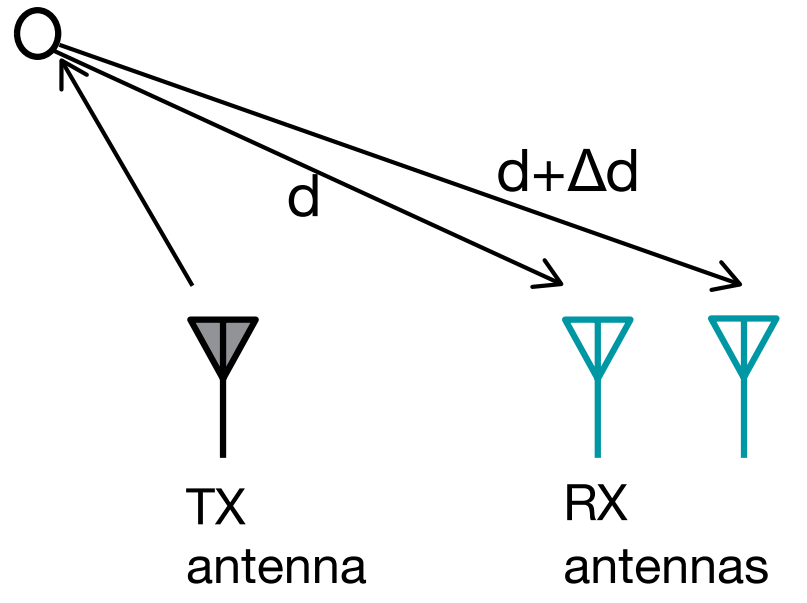
**Figure 9.** *Phase difference between RX chirps caused by angle offset of detected object.*

When a chirp is reflected off of the object, it has to travel a slightly longer distance to the second RX antenna than it does to the first. As seen in the velocity section, small differences in distance translate into large, linear differences in phase. Similar to velocity estimation, the phase difference between RX antenna 1 and RX antenna 2 can be measured and used to calculate the angle (also known as Azimuth) that the detected object is offset from the radar sensor. This same concept can be applied to localize the object in 3D. By adding a 3rd antenna below RX antennas 1 and 2, the difference in phase can be used to calculate the elevation angle.

The antenna count and shape has a significant impact on the sensors ability to localize objects. A higher number of antennas will typically increase the angular resolution of the sensor. For more information on how antenna design impacts the performance of a radar sensor, check out the Antenna Design module

How Does Radar Work?

Chirps

Range Estimation

Velocity Estimation

Detecting an object’s position

Product Enquiry